Fast Fourier Transform
The package xscale.spectral.fft provides easy and comprehensive functions
to estimate a multi-dimensional spectrum using the Fast Fourier Transform
(FFT). Out-of-core computation as well as parallelization are made possible
by using FFT functions from dask.array.fft.
Using multi-dimensional FFT
The spectrum over one or multiple dimensions of a xarray.DataArray
can be estimated with the FFT using the main function
xscale.spectral.fft.fft().
For a one-dimensional Fourier transform:
For a two-dimensional Fourier transform:
This function takes optionally the following parameters:
- Spectrum parameters
nfft: the number of points used for the FFTdim: the dimensions over which the FFT will be performeddx: the resolution of the dimensions ; if the resolution is not precised, it will be inferred from the dimensions associated with the data
- Data pre-processing
detrend: Precise the manner to detrend the datatapering: Multiply by aTukeywindow with a coefficient a 0.25
Note
- The parameters
nfft,dxare very flexible and may either be a number, a list/tuple or a dictionary. - Only the mean option is available for the moment to detrend the data before FFT computation.
- The
taperingoption is still experimental, it should be use with cautious
One dimensional FFT
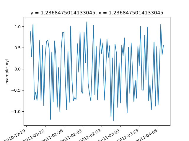
Let us start by importing a three-dimensional signal as an example:
In [1]: import xscale.signal.generator as xgen

In [2]: foo = xgen.example_xyt()

In [3]: foo
Out[3]:
<xarray.DataArray 'example_xyt' (time: 100, y: 128, x: 128)>
dask.array<shape=(100, 128, 128), dtype=float64, chunksize=(50, 70, 70)>
Coordinates:
  * time     (time) datetime64[ns] 2011-01-01 2011-01-02 2011-01-03 ...
  * y        (y) float64 0.0 0.04947 0.09895 0.1484 0.1979 0.2474 0.2968 ...
  * x        (x) float64 0.0 0.04947 0.09895 0.1484 0.1979 0.2474 0.2968 ...

In [4]: foo.isel(x=25, y=25).plot();
Here, we only want to estimate the spectrum along the time dimension, but
for every grid point.
In [5]: import xscale.spectral.fft as xfft

In [6]: foo_time_spectrum = xfft.fft(foo, dim='time', dx=1., detrend='mean',
   ...: tapering=True)
   ...:

In [7]: foo_time_spectrum
Out[7]:
<xarray.DataArray 'spectrum' (f_time: 51, y: 128, x: 128)>
dask.array<shape=(51, 128, 128), dtype=complex128, chunksize=(50, 70, 70)>
Coordinates:
  * y        (y) float64 0.0 0.04947 0.09895 0.1484 0.1979 0.2474 0.2968 ...
  * x        (x) float64 0.0 0.04947 0.09895 0.1484 0.1979 0.2474 0.2968 ...
  * f_time   (f_time) float64 0.0 0.01 0.02 0.03 0.04 0.05 0.06 0.07 0.08 ...
Attributes:
    ps_factor:   0.0002
    psd_factor:  0.02
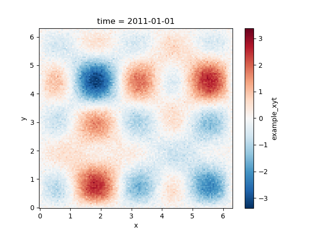
Two dimensional FFT
In [8]: foo.isel(time=0).plot();
In [9]: foo_yx_spectrum = xfft.fft(foo, dim=['y', 'x'], detrend='mean')

In [10]: foo_yx_spectrum
Out[10]:
<xarray.DataArray 'spectrum' (time: 100, f_y: 65, f_x: 128)>
dask.array<shape=(100, 65, 128), dtype=complex128, chunksize=(50, 65, 128)>
Coordinates:
  * f_x      (f_x) float64 -10.11 -9.948 -9.791 -9.633 -9.475 -9.317 -9.159 ...
  * f_y      (f_y) float64 0.0 0.1579 0.3158 0.4737 0.6316 0.7896 0.9475 ...
  * time     (time) datetime64[ns] 2011-01-01 2011-01-02 2011-01-03 ...
Attributes:
    ps_factor:   7.45058059692e-09
    psd_factor:  2.9878744956100273e-07
Spectrum normalization
The function xscale.spectral.fft.fft() returns a complex spectrum
\(S(f_x,f_y, t)\), which is not straightforward to interpret in a physical
sense. There exist several quantities and normalization that can be derived
from the complex spectrum, which are useful to give a physical interpretation to
the spectral estimates. We detail here the different quantities that
xscale.spectral.fft is able to compute. All normalization methods involve a
dask.array functions so that they can be easily combined with the FFT
computation to increment a dask graph.
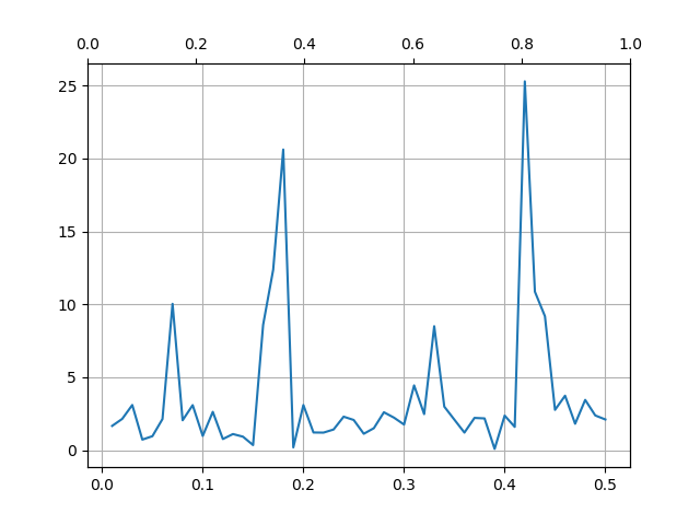
Amplitude spectrum
The amplitude spectrum is simply the squared sample modulus of the spectrum \(S\):
where \(\Re[S]\) and \(\Im[S]\) are the real and the imaginary parts of
the spectrum, respectively. The amplitude spectrum can be computed from the
previous example using the function xscale.spectral.fft.amplitude().
In [11]: from xscale.spectral.tools import plot_spectrum

In [12]: foo_time_amplitude = xfft.amplitude(foo_time_spectrum)

In [13]: foo_time_amplitude
Out[13]:
<xarray.DataArray 'spectrum' (f_time: 51, y: 128, x: 128)>
dask.array<shape=(51, 128, 128), dtype=float64, chunksize=(50, 70, 70)>
Coordinates:
  * y        (y) float64 0.0 0.04947 0.09895 0.1484 0.1979 0.2474 0.2968 ...
  * x        (x) float64 0.0 0.04947 0.09895 0.1484 0.1979 0.2474 0.2968 ...
  * f_time   (f_time) float64 0.0 0.01 0.02 0.03 0.04 0.05 0.06 0.07 0.08 ...

In [14]: plot_spectrum(foo_time_amplitude.isel(x=25, y=25));
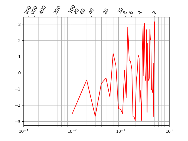
Phase spectrum
In [15]: foo_time_phase = xfft.phase(foo_time_spectrum)

In [16]: foo_time_phase
Out[16]:
<xarray.DataArray 'Phase Spectrum' (f_time: 51, y: 128, x: 128)>
dask.array<shape=(51, 128, 128), dtype=float64, chunksize=(50, 70, 70)>
Coordinates:
  * y        (y) float64 0.0 0.04947 0.09895 0.1484 0.1979 0.2474 0.2968 ...
  * x        (x) float64 0.0 0.04947 0.09895 0.1484 0.1979 0.2474 0.2968 ...
  * f_time   (f_time) float64 0.0 0.01 0.02 0.03 0.04 0.05 0.06 0.07 0.08 ...
Attributes:
    ps_factor:   0.0002
    psd_factor:  0.02

In [17]: plot_spectrum(foo_time_phase.isel(x=25, y=25), xlog=True, color='r');
Power spectrum (PS)
In [18]: foo_time_ps = xfft.ps(foo_time_spectrum)
In [19]: foo_time_ps
Out[19]:
<xarray.DataArray 'PS_spectrum' (f_time: 51, y: 128, x: 128)>
dask.array<shape=(51, 128, 128), dtype=float64, chunksize=(50, 70, 70)>
Coordinates:
* y (y) float64 0.0 0.04947 0.09895 0.1484 0.1979 0.2474 0.2968 ...
* x (x) float64 0.0 0.04947 0.09895 0.1484 0.1979 0.2474 0.2968 ...
* f_time (f_time) float64 0.0 0.01 0.02 0.03 0.04 0.05 0.06 0.07 0.08 ...
Attributes:
description: Power Spectrum (PS)
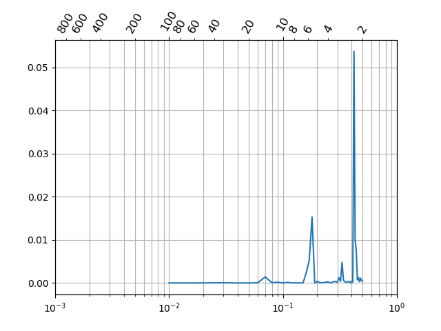
In [20]: plot_spectrum(foo_time_ps.isel(x=25, y=25), variance_preserving=True);
Power spectrum density (PSD)
In [21]: foo_time_psd = xfft.ps(foo_time_spectrum)
In [22]: foo_time_psd
Out[22]:
<xarray.DataArray 'PS_spectrum' (f_time: 51, y: 128, x: 128)>
dask.array<shape=(51, 128, 128), dtype=float64, chunksize=(50, 70, 70)>
Coordinates:
* y (y) float64 0.0 0.04947 0.09895 0.1484 0.1979 0.2474 0.2968 ...
* x (x) float64 0.0 0.04947 0.09895 0.1484 0.1979 0.2474 0.2968 ...
* f_time (f_time) float64 0.0 0.01 0.02 0.03 0.04 0.05 0.06 0.07 0.08 ...
Attributes:
description: Power Spectrum (PS)
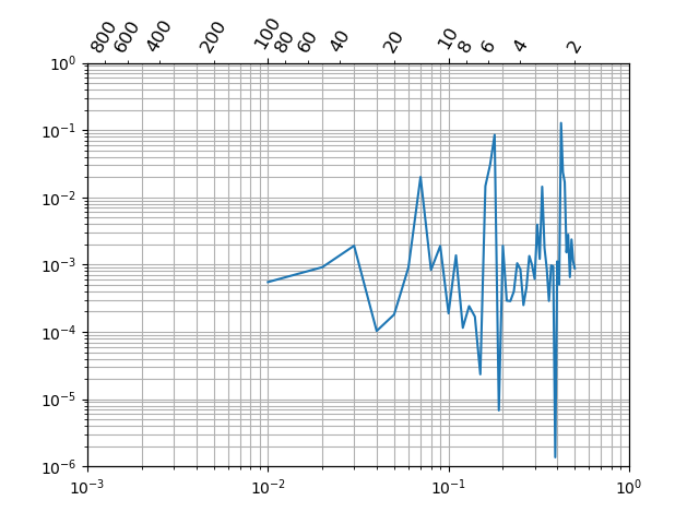
In [23]: plot_spectrum(foo_time_ps.isel(x=25, y=25), loglog=True);
Cross spectrum
This function is not implemented yet but will be available soon.