Fitting methods
This section describes different fitting techniques that uses parametric and non-parametric regression.
In [1]: import xscale.signal.fitting as xfit
Parametric methods
Polynomial fitting
Coming soon
Harmonic fitting
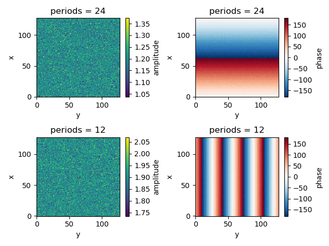
Harmonic fitting is used to capture periodic oscillation in the data when the oscillation periods \(T_k=1/f_k\) are known (where \(f_k\) is the frequency). The harmonic fitting is thus used to estimate the amplitude \(A_k\) and the phase \(\Phi_k\) of the oscillations.
For real data, the solution of the problem can be written:
For the least-square fit, it is common to use the cosine and sine form:
because the first problem is nonconvex and may have multiple minima. The equivalence between the two form is given by:
An idealized signal is built with two oscillations at 24 and 12 hours with a phase that depends on space:
In [2]: Nt, Nx, Ny = 100, 128, 128

In [3]: rand = xr.DataArray(np.random.rand(Nx, Ny, Nt), dims=['x', 'y', 'time'])

In [4]: rand = rand.assign_coords(time=pd.date_range(start='2011-01-01',
   ...:                                              periods=100, freq='H'))
   ...:

In [5]: offset = 0.4

In [6]: amp1, phi1 = 1.2, 0.

In [7]: wave1 = amp1 * np.sin(2 * np.pi * rand['time.hour'] / 24. +
   ...:                       phi1 * np.pi / 180 + 0.05 * rand.x)
   ...:

In [8]: amp2, phi2 = 1.9, 60.

In [9]: wave2 = amp2 * np.sin(2 * np.pi * rand['time.hour'] / 12. +
   ...:                       phi2 * np.pi / 180. + 0.2 * rand.y)
   ...:

In [10]: truth = offset + rand + wave1 + wave2

In [11]: truth = truth.chunk(chunks={'x': 50, 'y': 50, 'time': 20})

In [12]: fig, (ax1, ax2) = plt.subplots(2, 1)

In [13]: truth.isel(y=0).plot(ax=ax1)
Out[13]: <matplotlib.collections.QuadMesh at 0x7f15d1d5e710>

In [14]: truth.isel(x=0).plot(ax=ax2)
Out[14]: <matplotlib.collections.QuadMesh at 0x7f1603988990>

In [15]: plt.tight_layout()

In [16]: plt.show()

The fit is performed by using the xscale.signal.fitting.sinfit()
functions:
In [17]: fit2w = xfit.sinfit(truth, dim='time', periods=[24, 12], unit='h')

In [18]: print(fit2w)
<xarray.Dataset>
Dimensions:    (periods: 2, x: 128, y: 128)
Coordinates:
  * periods    (periods) int64 24 12
  * x          (x) int64 0 1 2 3 4 5 6 7 8 9 10 11 12 13 14 15 16 17 18 19 ...
  * y          (y) int64 0 1 2 3 4 5 6 7 8 9 10 11 12 13 14 15 16 17 18 19 ...
Data variables:
    phase      (periods, x, y) float64 dask.array<shape=(2, 128, 128), chunksize=(2, 16, 128)>
    amplitude  (periods, x, y) float64 dask.array<shape=(2, 128, 128), chunksize=(2, 16, 128)>
    offset     (x, y) float64 dask.array<shape=(128, 128), chunksize=(16, 128)>
In [19]: fig, ((ax1, ax2), (ax3, ax4)) = plt.subplots(2, 2)

In [20]: fit2w.sel(periods=24)['amplitude'].plot(ax=ax1)
Out[20]: <matplotlib.collections.QuadMesh at 0x7f1603357410>

In [21]: fit2w.sel(periods=24)['phase'].plot(ax=ax2)
Out[21]: <matplotlib.collections.QuadMesh at 0x7f1603352c50>

In [22]: fit2w.sel(periods=12)['amplitude'].plot(ax=ax3)
Out[22]: <matplotlib.collections.QuadMesh at 0x7f16068b7350>

In [23]: fit2w.sel(periods=12)['phase'].plot(ax=ax4)
Out[23]: <matplotlib.collections.QuadMesh at 0x7f16038c0490>

In [24]: plt.tight_layout()

In [25]: plt.show()
In [26]: rec = xfit.sinval(fit2w, truth.time)

In [27]: print(rec)
<xarray.DataArray (time: 100, x: 128, y: 128)>
dask.array<shape=(100, 128, 128), dtype=float64, chunksize=(100, 16, 128)>
Coordinates:
  * y        (y) int64 0 1 2 3 4 5 6 7 8 9 10 11 12 13 14 15 16 17 18 19 20 ...
  * x        (x) int64 0 1 2 3 4 5 6 7 8 9 10 11 12 13 14 15 16 17 18 19 20 ...
  * time     (time) datetime64[ns] 2011-01-01 2011-01-01T01:00:00 ...
    periods  int64 24

In [28]: rec12 = xfit.sinval(fit2w.sel(periods=[12,]), truth.time)

In [29]: rec24 = xfit.sinval(fit2w.sel(periods=[24,]), truth.time)
In [30]: truth.isel(x=10, y=10).plot(label='Truth')
Out[30]: [<matplotlib.lines.Line2D at 0x7f15d1a8d790>]

In [31]: rec.isel(x=10, y=10).plot(label='Recontruction with 2 modes')
Out[31]: [<matplotlib.lines.Line2D at 0x7f16038c8fd0>]

In [32]: rec24.isel(x=10, y=10).plot(label='Recontruction with mode 1, T=24h',
   ....: ls='--')
   ....:
Out[32]: [<matplotlib.lines.Line2D at 0x7f1606551b50>]

In [33]: rec12.isel(x=10, y=10).plot(label='Recontruction with mode 2, T=12h',
   ....: ls='--')
   ....:
Out[33]: [<matplotlib.lines.Line2D at 0x7f16038f6090>]

In [34]: plt.legend()
Out[34]: <matplotlib.legend.Legend at 0x7f16033de450>

In [35]: plt.show()

Note
For complex signals, the harmonic fitting is not available yet. This should be done for future versions
Exponential fitting
Coming soon